Simulation Timing
In this post, we will explain our understanding of simulation frames and their correlation to the real-world’s linear time we all live in.
Simulation Frame
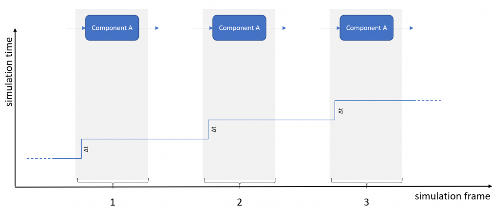
A component’s simulation frame consists of all internal steps that are required to compute and provide an output from a given input. In time-based simulation applications (as is the case for most systems used in environment simulation solutions) a frame corresponds to a specific progress in simulation time, or, a time interval.
The following figure illustrates this process. Simulation time is progressing in discrete steps, i.e., by the delta time that a component’s calculations are supposed to represent. If all steps (or frames) of a simulation represent identical delta time, the system is considered a “fixed-step system” or “fixed-step solver”.
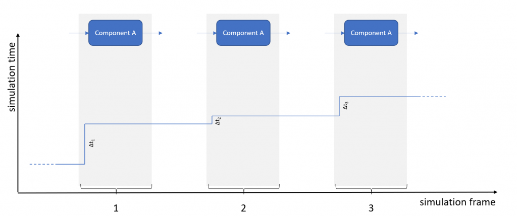
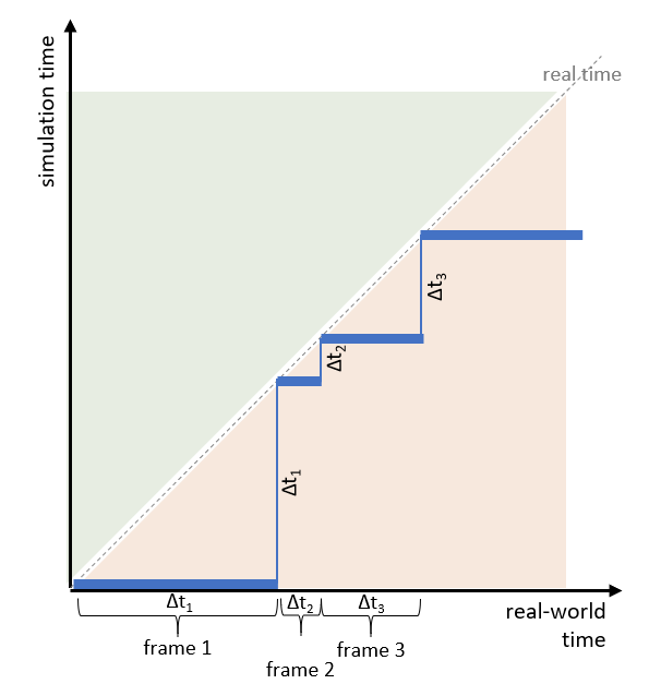
Applications may also allow for non-constant, i.e., variable steps. In that case, the previous chart changes slightly:
The (maximum) size of a simulation step (in fixed- and variable-step mode) is given by limiting factors in precision and stability. Controllers and integrators (linear and non-linear) tend to become unstable if the steps are too large. On the other hand, if your simulation steps are too small, you may achieve great precision but you will lose precious computation time and, thus, money (or your competitive edge).
Realtime and Non-Realtime Operation
One of the key criteria in our ratings is the ability of a system to run in real-time or non real-time mode. There are, basically, three operating modes available:
- slower than real time
- real time
- faster than real time
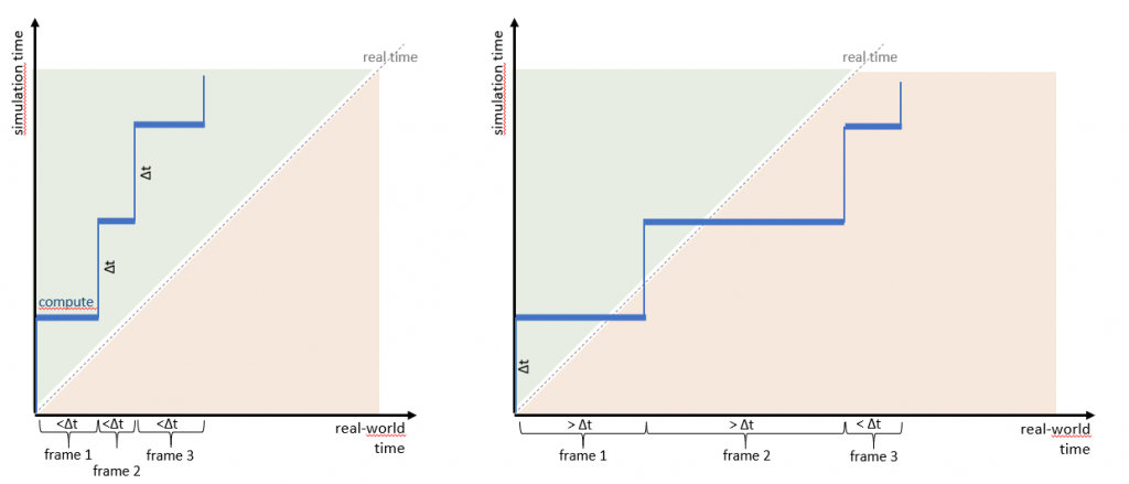
These terms describe how the simulation time – the sum of the delta times per simulation step – “accumulates” relative to the time in the real world:
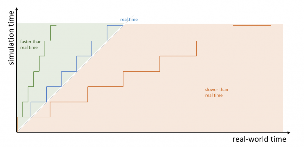
In the figure above, the delta time of each simulation step is identical (fixed-step solver) but the real-world time between the steps differs and, therefore, influences the correlation between simulation time and real-world time. A system that accumulates simulation time in-sync with the progress of real-world time is called a real-time system. Systems where simulation time accumulates faster or slower than real-world time are labeled accordingly.
Note (don’t read if you’re already confused): when talking about real time in the following paragraphs, we usually mean real time with a factor of one. There may be systems requiring to run in exact multiples (or fractions) of real time – twice real time, for example – but since this only implies multiplying the real-world time with a factor, everything else we will be saying about the correlation between simulation time and real time remains valid.
Compute Time vs Idle Time
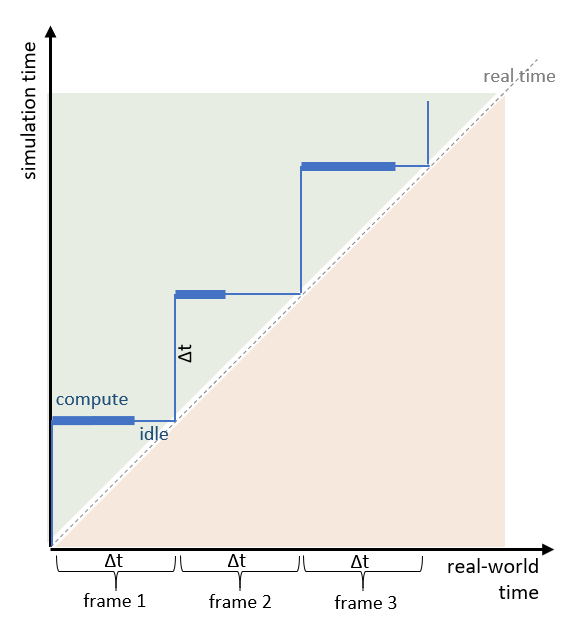
Not all the real-world time that passes between two simulation frames has to be used for actually computing a frame – and it shouldn’t. If you want to stay withing real-time constraints, your system’s compute time has to stay below the full duration of the step, so that you can trigger the next frame in due time. It doesn’t matter whether your compute time differs between frames as long as you keep it lower than the simulation time step it is aimed to represent. This is indicated by the following figure (note: simulation time matches real time a the end of each frame):
Go as Fast as Possible
If you get rid of all idle times, your system will run as fast as possible and its correlation to real time will depend only on the simulation step size (frame time) and the compute time required for calculating a step. This may be real time (quite an exception) or faster or slower. Since your compute times may vary for each simulation step (eg, due to different components being updated in different steps), a fixed-step system may appear quite “jittery” (see following figure):
Increasing the speed of simulation execution in the go-as-fast-as-possible setup can only be achieved in two ways, by reducing the compute time (eg, by optimizing your algorithms, parallel execution, or using a more powerful computer) or by increasing the simulation step size (ie, more simulation time gets done per step). However, as indicated above, always keep in mind that systems may lose precision and/or stability if you reduce the granularity of the calculations. There will always be a maximum simulation step size beyond which it may the the fastest not to perform any simulation at all because results become useless anyway.
Struggling With Real Time
Installations with real (target) hardware or humans-in-the-loop require that simulation time progress along real-world time. As indicated above, the best way to guarantee this is to make sure that your actual compute time is lower than the time step it represents. You may add a (variable) bit of idling at the end of your simulation frame and will then be able to start the next frame right on the spot.
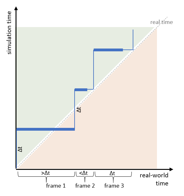
But what to do if your system takes longer to compute a simulation step? Let’s take a look at the following figure:
In this example, the first and second frames’ compute times are longer than the nominal frame time (which is identical with the simulation step). As is the case with many real-time-capable systems, the system is laid out in a way that frames are only executed at clear boundaries that correspond to multiples of the simulation step size (Δt). Therefore, if a frame’s computation takes too long, the system will idle until the next boundary becomes available. A visual system, for example, will run nominally at 120Hz, but may slow down to 60Hz or 30Hz with increasing load.
If the timing is done as in the figure above, it means that your simulation time is continuously falling behind (you need 2x Δt to compute a step of Δt) and that you are, thus, operating slower than real time. This is not acceptable if other components in your setup depend on real-time operation and if long frames are more than just a rare exception.
Keeping up With Real Time
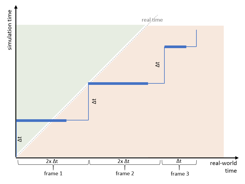
One way to keep up with real time is to skip frames so that, overall, real time is preserved. The following figure illustrates this frame drop:
After detecting an overrun of a frame, the system skips the next frame and increases the simulation step size for the (new) next frame. By this, the system will temporarily be out of real time but will realign with the upcoming frame. A complete frame’s results, though, are skipped.
This method may appear like a nice, scalable solution; but it may irritate components which depend on your simulator providing results in due time. In an interactive driving simulator, for example, it will appear to the human spectator as though the system got stuck for a very short moment and will, thus, deteriorate the immersion that is necessary for this kind of simulator (and may, in the worst case, be one of the causes for simulator sickness). Also keep in mind that increasing the simulation step size may result in less precise computations or even instabilities of controllers.
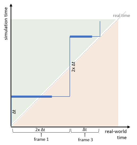
If your system is laid out in a way that long frames are followed by short ones, a single overrun may be “healed” by an upcoming frame (not necessarily the direct successor):
If long frames are a rare event, other components depending on your simulation may get along with the noise introduced by this behavior. But this is nothing you should rely on and you’d better work on getting rid of long frames in the first place.
Variable Frames and Real Time
With variable simulation frames, you might be in a much better position to react on different execution times and keep real-time operation. You may either operate completely without idle time (ie, your simulation steps may become as short as it takes to compute them) or with an optional idle time so that your frames don’t become too short. The following figure illustrates an adaptive real-time operation without idle times:
In this case, the simulation time represented by a frame depends on the computation time (real-world time) it took to compute the previous frame. Therefore, real time is achieved at the beginning of a successor frame, not at the end of an actual frame.
Note: Whether simulation time and real-world time have to correspond at the beginning or end of a frame in real-time operation, is another question, that may lead to “interesting” discussions. It pretty much depends on how you consider the computation of frame 0. Does it start with zero time increment and computes a dummy frame (as in the figure above) or does it already include the first simulation step increment (as in all other figures higher above). We’ll leave that decision to you.
Summary
What are the key takeaways of this post?
- Simulation comes in discrete frames (steps)
- Simulation steps must not be too large in order to avoid instability and inaccuracies
- Steps consist of compute time and – optionally – idle time
- In a real-time system, simulation time progresses in sync with real-world time
- The compute time in real-time systems has to be lower than the step size
- Real-time systems have to be monitored for overruns and frame drops
- Overruns and frame drops have to be compensated for
- Jitter and noise induced by frame drops, overruns, or variable step sizes are to be avoided, especially when working under real-time conditions with hardware- or humans-in-the-loop
Outlook: Timing Across Various Components
In this post, we treated a simulation instance as a quite rigid, single component. Many solutions, however, are composed of various components that need to be kept aligned with some kind of reference timing. Read more about alignment and synchronization in a dedicated post.