Simulation Synchronization
Synchronizing various components that belong to a simulation system may range between trivial and tricky. In this post, we will shed some light on common methods and technologies of simulation synchronization. If you are not familiar yet with the basics of simulation timing, it might be a good idea to read our dedicated post on this subject first.
Our System
Let’s take a system as we often find it in simulation applications for Advanced Driver Assist Systems or Automated Driving (for more details on this subject, please go here):
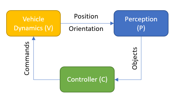
We have a Vehicle Dynamics (V) component that computes the position and orientation of the vehicle based on the input by the Controller (C). The Controller computes its commands based on information which it receives from the Perception System (P). And the perception depends on the sensors’ positions and orientations which are, to close the loop, depending on the vehicle’s state. BTW: in a driver-in-the-loop system, another perception and control layer will be provided by the human driver. But let’s keep things simple for now.
Everything is In-Sync and In-Line
The easiest case is a fully synchronized system where each component starts computing after the previous component has provided its results:
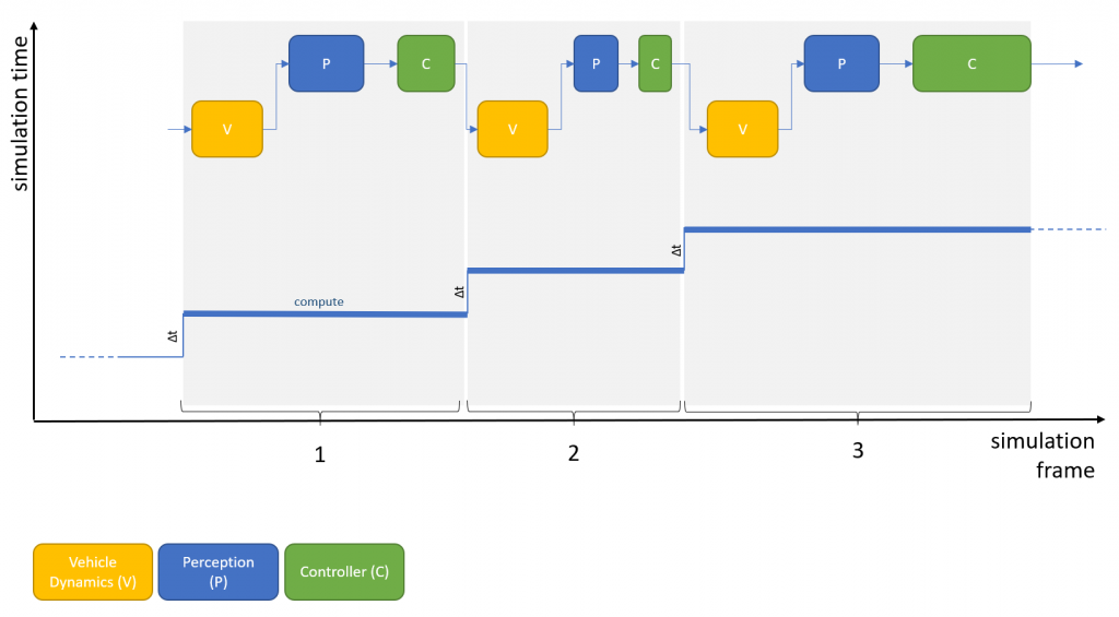
In our system, we assume fixed steps, so that the delta simulation time in each simulation step (or frame) is identical (see simulation time graph in the figure). The overall execution speed of the system – as depicted in the figure above – depends only on the speed of the components (note that the frames need different compute times to calculate simulation time steps of identical size; this may be due to a component’s internal calculations changing between steps). Again, for more information on timing, see our post “Simulation Timing“.
In-Sync with Varying Granularity
Some components may require smaller simulation time steps in order to achieve a certain accuracy and/or to avoid instabilities in internal integrators or controllers. In our test system, the most “sensitive” component is the Vehicle Dynamics (V). If we introduce subsampling for this component, the previous figure changes slightly:
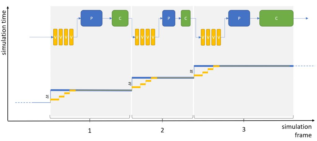
Overall, the behavior of the system does not change and the sequence of events is the same as before. Just the accuracy of the vehicle dynamics may have increased (the vehicle dynamics may, for example, query road contact points more frequently in order to compute the tire model).
In-Sync with Parallel Execution and Varying Granularity
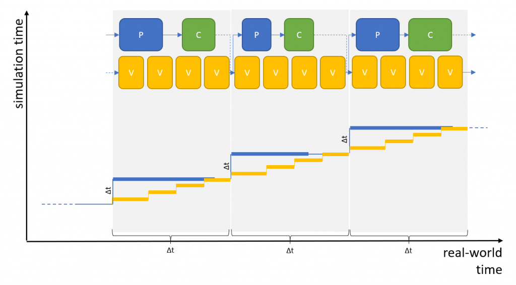
Our system may run faster if we make use of the fact that our perception and controller components may not need the very latest results of the vehicle dynamics component but may live as well with the previous frame’s results. In this case, we can save the time it takes for the vehicle dynamics to compute its results and we can kick it off in parallel:
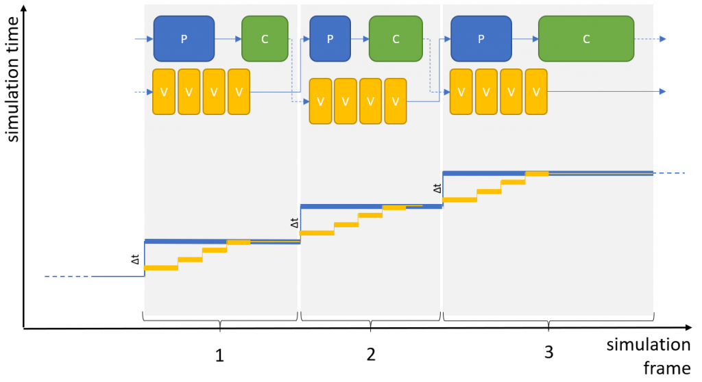
Of course, we add one frame latency to the system by this setup and it is up to the user to decide whether a system can handle this offset in timing. On the other hand, we will save some time per simulation frame and this will enable us to run our simulation faster or with increased granularity.
Going Real Time in Full Sync
The systems described so far have all been non-real-time systems. They run as fast as the slowest chain of components allows. But in Hardware- or Driver-in-the-Loop (HiL / DiL) systems – just to name a few – real time is the only way to go. In these setups, components (or humans) are involved which cannot tolerate a simulation time that progresses different from the real-world time (although it will progress in steps, of course, not continuously).
Therefore, let’s take a look at a real-time systems that runs in full sync (note that in the upcoming figures, the horizontal axis is showing real-world time instead of frames, and that the scaling of simulation time and real-world time differs for better illustration, i.e., Δt intervals on the horizontal and vertical axis are of identical duration):
If you go with full sync in real time you have to identify a base frame time – typically the one of the component with highest granularity – and align all components to integer multiples of this frame time. Components, or chains of components, that finish “early” will have to idle until the next frame boundary.
This setup works pretty nicely if you can guarantee that components do not exceed their allocated frame times and that all frame times add up correctly for each simulation frame.
Real Time in Asynchronous Operation
If your components run completely independently and/or their frame times don’t match a multiple of a basic frame time (imagine a 120Hz component running at 8.33ms and a 1kHz component running at 1ms), you have to go to asynchronous operation. The key to this mode is that all components agree on a common time domain and progress simulation time according to this domain. In most applications, the underlying time domain is the real-world time and all components will run in real time.
Theoretically, you may choose another time domain or multiples of real time but this is a rather rare use case.
Your system will now operate as shown in the following figure:
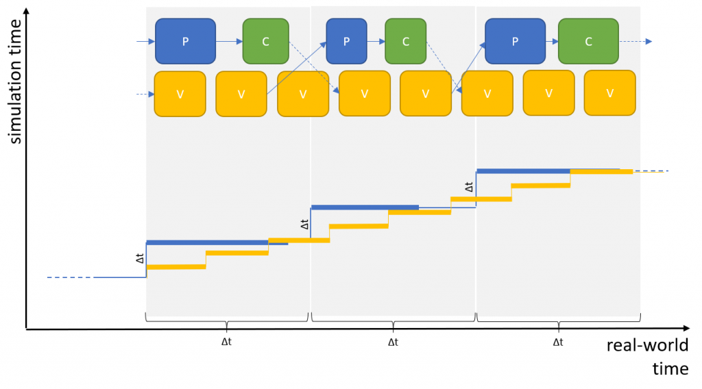
As can be seen from the figure, the inputs to the Perception (P) and Vehice Dynamics (V) components will be based on the latest available results of the respective components. The “age” of these results may vary from frame to frame (sometimes two, sometimes three cycles of V are computed as input to P in our example).
This means that components may not be able to use inputs as they are but that they have to align these inputs with their own, internal time stamp. For discrete inputs – like the state of a switch – there is no need to perform any additional calculation. But for continuous inputs like position, orientation, speed etc. there may be a need to “predict” the values corresponding to a consuming component’s internal time stamp based on the arbitrarily “old” results of the providing component.
This can be done if you have knowledge about the gradients of a continuous input (e.g., by using speed to predict position) and if you have knowledge about the precise time stamps for which the input has been calculated (note: this only works because we have agreed on a common time base – real time – as described before).
Whether gradients are computed and provided by the component that provides the actual input or whether the receiver of the input keeps an internal history and computes gradients by itself is a matter of system design (and accuracy, of course). But the source of the gradients does not affect how you have to handle and align asynchronously computed results.
Summary
In this post, we tried to highlight the key elements of synchronization between different components in a simulation system. Many systems will work in synchronous operation mode with fully or partially sequential execution including components of varying granularity. But when it comes to running real-time systems with a series of components whose frame times do not fully match up, asynchronous operation is the way to go.